Implementation details: From the original Transformer to GPT

1 The original Transformer reviewed

1.1 Attention block

1.1.1 Scaled dot-product attention

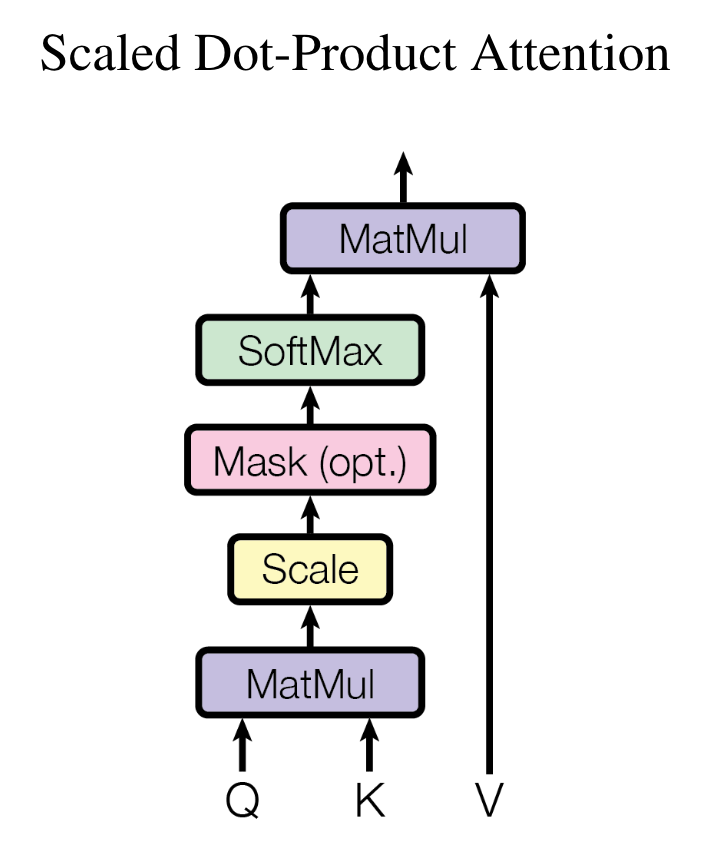
• Query and the attention output are one-to-one mapped. For each query (a vector), we compute one output.
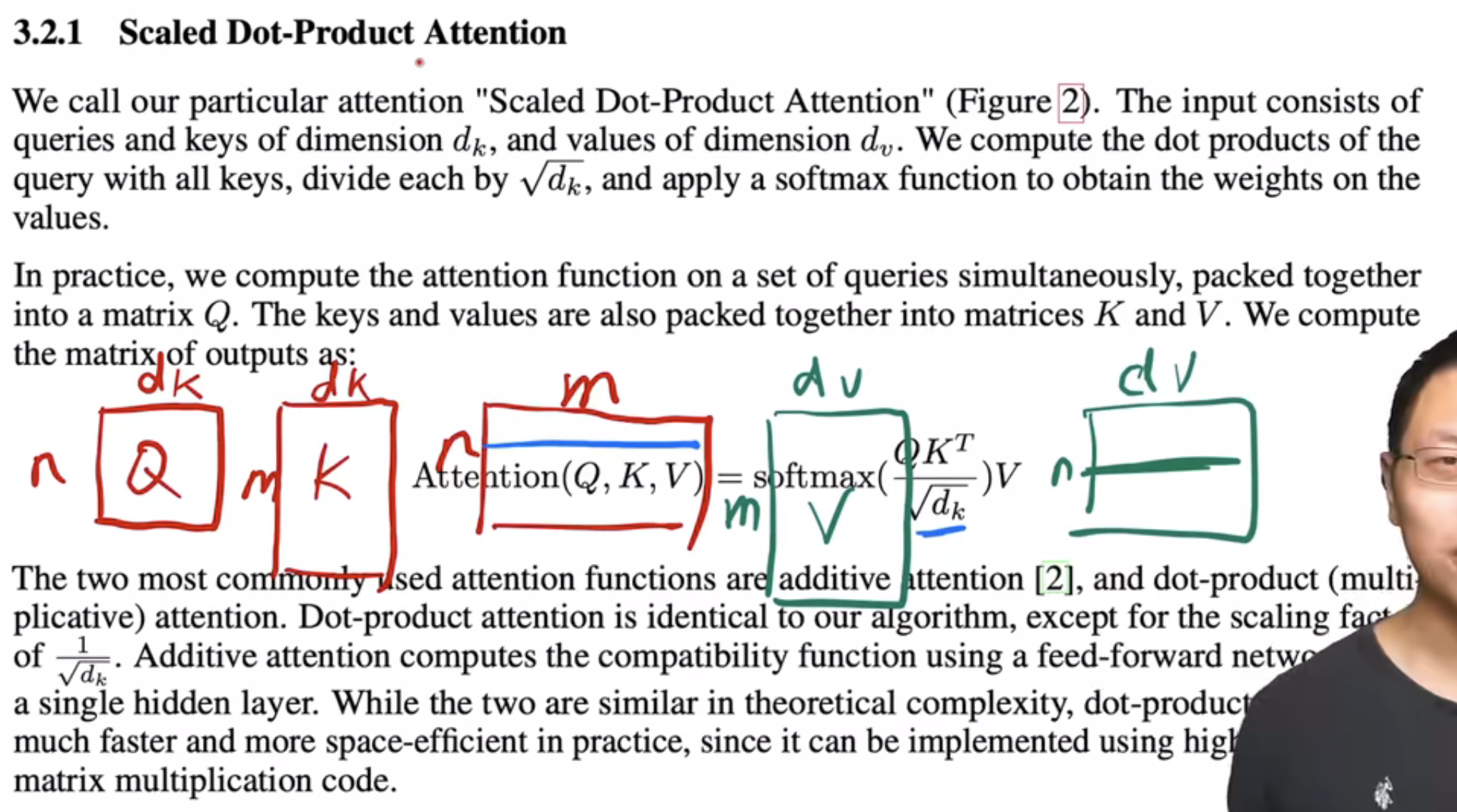
  • So, if we have $n$ queries (i.e., $Q$ is $n\times d$), the output is $n\times d$.
  • The output for each query is a weighted sum of values.
• Softmax is applied to the rows of $QK^T$, i.e., $\sum_j \text{softmax}(QK^T)_{i,j}=1$.

Why divide by $\sqrt{d_{k}}$?

When we compute $QK^T$, we compute many vector dot products of size $d_k$. When $d_k$ is large (e.g., 512, 4096), the variance of the result becomes large. Selecting a row (recall softmax is row-wise) of $QK^T$, some elements are very small while others are very large. If we apply softmax on this row, the result will be skewed toward 0 or 1.

This leads to small gradient updates. You can see the gradient at the two sides of a sigmoid function is close to zero:

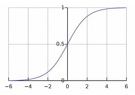
Dividing by $\sqrt{d_k}$ keeps the softmax inputs closer to the center of the distribution, leading to larger gradients.

The brief explanation from the authors is:

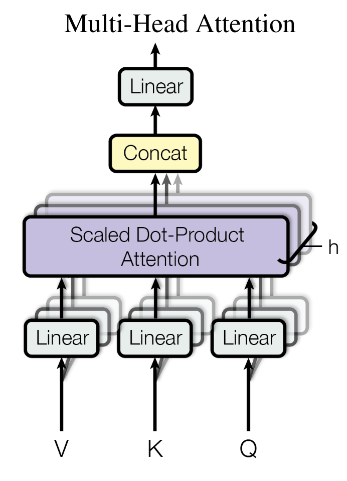
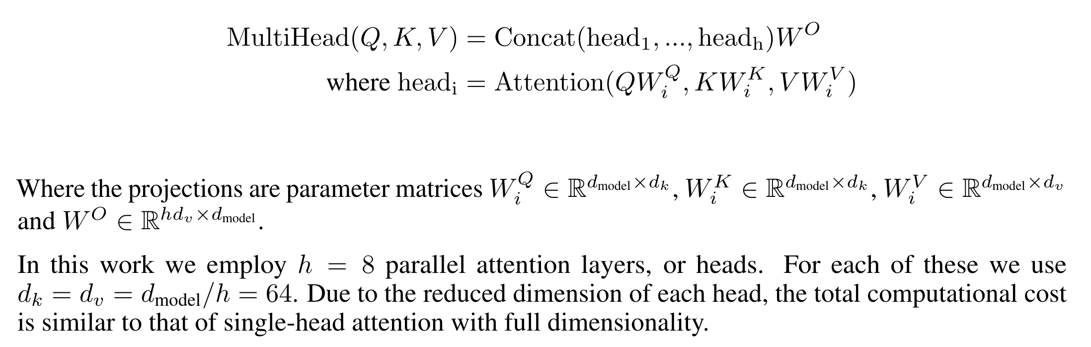
1.1.2 Multi-head attention (MHA)

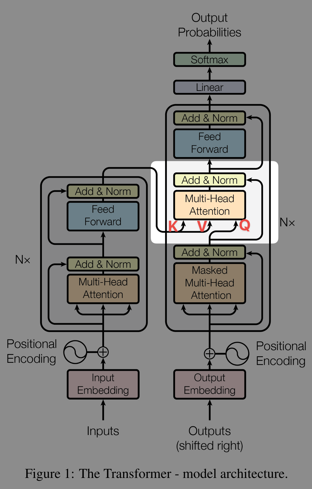
1.1.3 Cross attention (Encoder & decoder)

1.2 FFN block

FFN is simply an MLP applied to the last dimension. The output of the attention block is $n\times d_k$ where $n$ is the sequence length (number of tokens). Let $x$ be the embedding of one token (a vector). FFN does: $$ \operatorname{FFN}(x)=\max(0,xW_{1}+b_{1})W_{2}+b_{2} $$ $W_{1}$ projects from $d_k$ to $4\times d_k$, and $W_{2}$ projects it back to $d_k$.

1.3 Embedding and positional encoding

• In the original paper, the authors use the same embedding matrix in three places: 1) encoder, 2) decoder, and 3) the final FF layer before softmax (where for each token you produce $V$ logits, with $V$ the vocabulary size)
  • embedding matrix: $V\times d_{model}$
• The authors also multiply the embedding matrix by $\sqrt{d_{model}}$.
  • After training, the $\ell_2$ norm of an embedding vector is usually very small and does not increase with $d_{model}$. For example, when $d_{model}$ increases from 512 to 4096, the $\ell_2$ norm of the embedding may still be ~1.
  • However, the $\ell_2$ norm of positional encoding increases with length.
  • So, if we do not scale the embedding, it will be dominated by the positional encoding when added.

1.4 Dropout

• Residual dropout: before adding to the sublayer input (see “Drop1” and “Drop2” in the pre-LN example below; “Drop” is for FFN)
  • x + Drop1(MHA(LN(x))) (Attention sublayer)
  • x + Drop2(Linear2(Drop(activation(Linear1(LN(x)))))) (FFN sublayer)
• Attention dropout:
  • Applied after softmax, before multiplying V (i.e., on the attention weights).
  • $\operatorname{Drop}\left(\operatorname{Softmax}\left( \frac{QK^T}{\sqrt{d_k}}\right) \right)V$
• Embedding dropout: after summing embedding and positional encoding
  • Drop(input_embed + pos_enc)
• FFN dropout: only for the hidden layer in FFN.

1.5 LayerNorm

• There are two variants: pre-LN and post-LN. In the original Transformer, the authors use post-norm, but GPT and later models prefer pre-LN.
• Pre-LN makes gradients smoother; see Xiong et al. (2020).

# pre-norm (preferred)
x = x + MHA(LN(x))
x = x + FFN(LN(x))

# post-norm
x = LN(x + MHA(x))
x = LN(x + FFN(x))

2 PyTorch implementation of Transformer

last update: pytorch-2.0.1

2.1 Config

• norm_first: If True, use pre-norm. Default: False (post-norm).
• dim_feedforward: default=2048
• activation: Default “relu”
• dropout: Default 0.1

2.2 Encoder

# How TransformerEncoderLayer.forward works

# x: input source
# Drop1, Drop2: residual dropout
# Drop: FFN dropout
# note: SA() doesn't include any dropout layer

# Pre-LN (preferred)
x = x + Drop1(SA(LN(x)))  # Self-Attn sublayer
x = x + Drop2(Linear2(Drop(Activation(Linear1(LN(x))))))  # FFN sublayer

# Post-LN
x = LN(x + Drop1(SA(x)))  # Self-Attn sublayer
x = LN(x + Drop2(Linear2(Drop(Activation(Linear1(x))))))  # FFN sublayer

2.3 Decoder

# How DecoderLayer.forward works

# x: the "Q"
# memory: the "K and V", from encoder
# Drop1, Drop2, Drop3: residual dropout
# Drop: FFN dropout
# note: SA() and MHA() don't include any dropout layer

# Pre-LN (preferred)
x = x + Drop1(SA(LN1(x)))  # SA sublayer
x = x + Drop2(MHA(LN2(x), memory))  # Multi-Head Attn
x = x + Drop3(Linear2(Drop(Activation(Linear1(LN3(x))))))  # FFN sublayer

# Post-LN
x = LN1(x + Drop1(SA(x)))  # SA
x = LN2(x + Drop2(MHA(x, memory)))  # MHA
x = LN3(x + Drop3(Linear2(Drop(Activation(Linear1(x))))))  # FFN sublayer

3 Compare with GPT

Below, I show how GPTs differ from the original Transformer. Since the GPT family is not open-source, the GPT code is from Hugging Face’s implementation of GPT-2. OpenAI reports GPT-3 uses the same architecture as GPT-2, except for the Sparse Transformer part.

3.1 Tokenizer: A variant of BPE

• Works on bytes, but avoids merges across character categories (e.g., punctuation and letters are not allowed to merge), except for spaces.
• e.g., "Hello world" => ["Hello", " world"]. Notice the leading space before “world.”

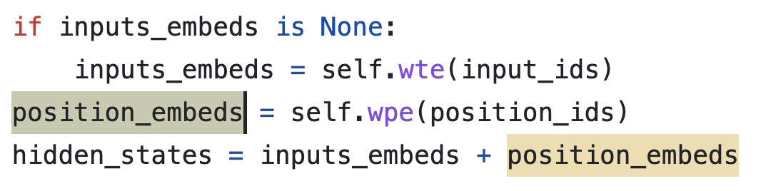
3.2 Embedding & positional encoding

• Both are learned

  

• Embedding is not scaled before adding to positional encoding (PE)
  • In the original Transformer, input_embeds is multiplied by $\sqrt{d_{model}}$. That’s because PE is based on sin/cos (not learned) and its $\ell_2$ norm increases with $d_{model}$.
  • But in GPT, PE is learned. Therefore, PE and input embeddings can be of similar scale.

    

3.3 LayerNorm

• Uses pre-LN.
• Another LN is added after the final attention block.

# first go through the blocks
for block in DecoderList:
    x = block(x)

# the final LN before output!
output = LN(x) 

3.4 Dropout

• GPTs have dropout in residual, embedding, and attention, same as the original Transformer (drop=0.1).
• GPT has no dropout in FFN.

  

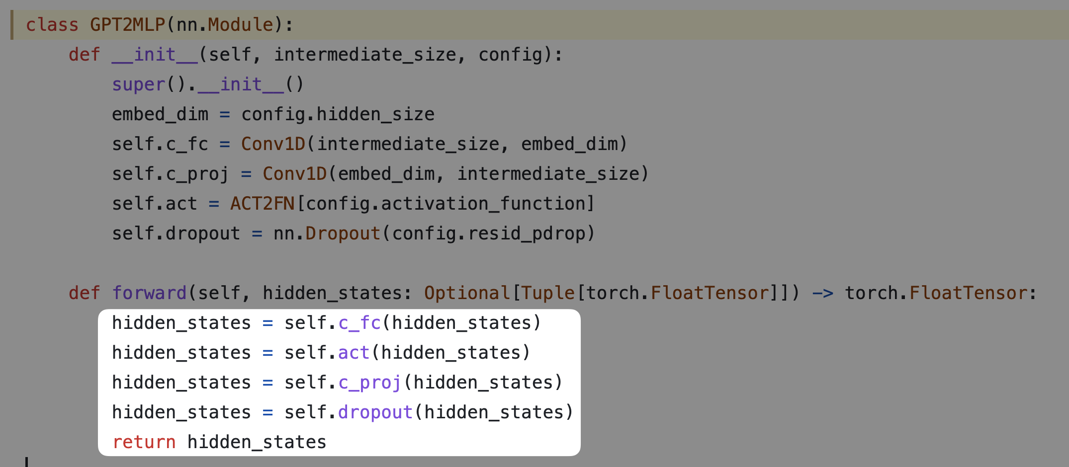
3.5 Activation: GELU

(Hendrycks & Gimpel, 2016) $$ \text{GELU} = x\Phi(x) $$ where $\Phi(x)$ is the CDF of the normal distribution. A common approximation is: $$ 0.5, x, \Big( 1 + \tanh\big[ \sqrt{2/\pi},(x+0.044715x^3)\big] \Big) $$

def gelu(self, input: Tensor) -> Tensor:
    return 0.5 * input * (1.0 + torch.tanh(math.sqrt(2.0 / math.pi) * (input + 0.044715 * torch.pow(input, 3.0))))

3.6 Initialization

• Linear and conv1d are normal with mean=0, std=0.02.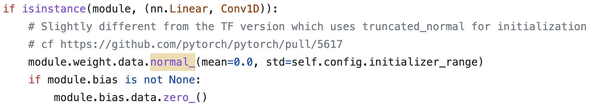

  

• Embedding and PE are normal with mean=0, std=0.02; padding_idx is 0.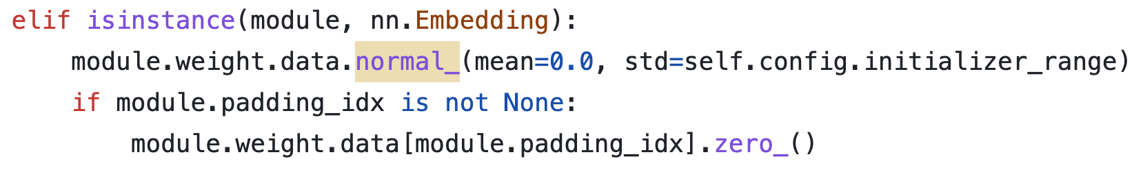

  

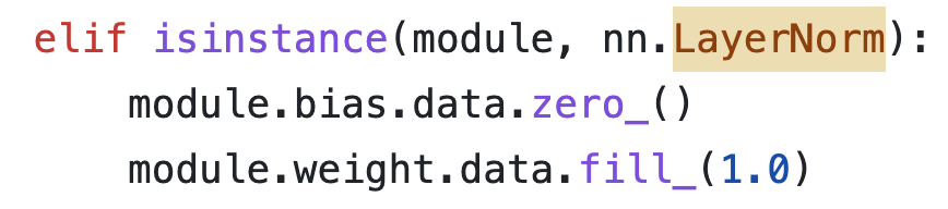
• LayerNorm has no affine transformation.

  

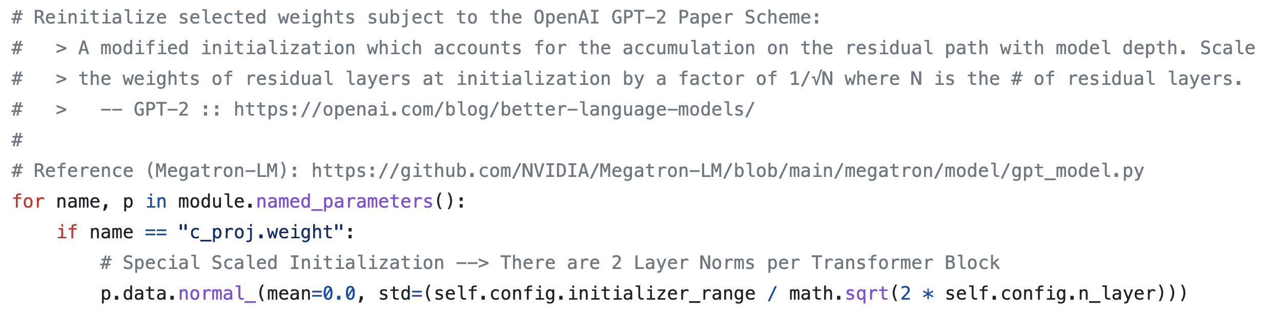
• (Important) Reinitialize selected weights
  • c_proj is the $W^O$ matrix in the original paper, sized $d_{model}\times d_{model}$. The concatenated attention outputs are multiplied by $W^O$ before the residual.
  • I still do not fully understand why “training signals accumulate through the residual path.”