Synthetic Control

1 Constructing of a synthetic control

The following explanation is adpted from (Abadie et al., 2010).

$Y_{it}$ is the outcome where $i=1,\dots,J+1$ and $t=1,\dots,T$. $Y_{it}^N$ and $Y_{it}^I$ are counterfactual outcome for the untreated and treated. The treated group is denoted by $i=1$ and the control groups (the “donor pool”) are denoted by $i=2,\dots J+1$. The treatment is applied on $T_{0}$ where $1\leq T_{0}<T$.

$W$ is a $(J\times 1)$ vector $(w_{2},w_{3},\dots,w_{J+1})’$ with nonnegative elements. The synthetic control at time $t$ is produced by $\sum_{j=2}^{J+1} w_{j}Y_{jt}^N$. The treatment effect at $t$ is $Y_{1t}^I - \sum_{j=2}^{J+1} w_{j}Y_{jt}^N$.

As you can see, the key procedure is to estimate $W$. Consider a $(k\times 1)$ vector $X_{1}=(Z_{1}, Y_{1}^{(1)}, Y_{1}^{(2)},\dots,Y_{1}^{(m)})$. $Z_{1}$ is a vector of covariates for the treated. Typically, they’re predictors of $Y_{1}$. $Y_{1}^{(m)}$ is a combination of pre-treatment $Y_{1}$. The most obvious choice is $Y_{1}^{(1)}=Y_{11}, \dots, Y_{1}^{(m)}=Y_{1T_{0}}$, i.e., the $Y_{1t}$ in every pre-treatment year. Conceptually, $X_{1}$ captures the characteristics of the treated. Note that there’s no $t$ subscript in $X_{1}$, indicating it’s an average over the pre-treatment periods. For example, if $Z_{1}$ could be the average per-capita GDP during the pre-treatment years.

Now consider another $(k\times J)$ matrix $X_{0}$. $X_{0}$ is similar to $X_{1}$ but it captures the characteristics of all units in the donor pool. Our weight $W$ is given by minimizing:

i.e., minimizing the characteristics between the treated and the synthetic control. $V$ is typically a semi-positive diagonal matrix whose elements determines the importance of each covariate in $X$. $V$ is typically given by:

where $Z$ is the pre-treatment trajectory of $Y$, i.e., $Z_{1}=(Y_{11},\dots,Y_{1T_{0}})$. So basically Eq(2) says $V$ is determined by minimizing the prediction error of the outcome.

Now you know how to estimate $W$ and $V$, the rest is straightforward.

2 Placebo falsification

2.1 Placebo “states”

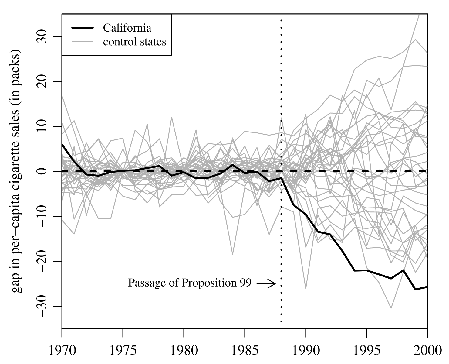
One can fixed the treatment dates but randomly shuffle the treatment states. In the California Proposition 99 case (Abadie et al., 2010), the treatment date is 1988, the treated state is California, and there’s a donor pool. To do a placebo falsification, the authors:

“In each iteration we reassign in our data the tobacco control intervention to one of the 38 control states, shifting California to the donor pool. That is, we proceed as if one of the states in the donor pool would have passed a large-scale tobacco control program in 1988, instead of California.”

Then, the author re-estimate the model and plot the real and synthetic cigarette consumption before and after the treatment data:

As can be seen from the figure, California is in the “extremely negative side” of the scale.

For a numerical test of the results conveyed in the above figure, one can:

1. Calculate the pre-treatment prediction error (i.e., $\sum_{t=0}^{T_{0}} (Y_{1t}-\sum_{j=2}^{J+1} w_{j}Y_{jt})^2$, measured in MSE)
2. Similarly, calculate the post-treatment prediction error.
3. Calculate the ratio of post- to pre-treatment MSE
4. Now you have a distribution of ratios, you can compute p-value of the treated state.

2.2 Placebo “dates”

When we do a placebo date, we keep the treated and untreated states fixed, but each time choose a different treatment date. Usually, the placebo dates are dates before the treatment date (i.e., we rewind the time). An example is Abadie, Diamond, and Hainmueller (2015).