Difference-in-Differences
1 DD model
The basic setting is: $$Y_{ist}=\alpha+\lambda_{s}+\lambda_{t}+\delta\times Treat_{s}\times Post_{t}+\beta X_{it}+\varepsilon_{it}$$
- $i$, $s$, and $t$ represent unit (e.g., person), group (e.g., state), and time (e.g., year).
- $Treat_{s}$ is a dummy equal to 1 if $s$ belongs to the treatment group. $Post_{t}$ is a dummy equal to 1 if $t$ is post‑treatment.
- $\lambda_{s}$ and $\lambda_{t}$ are fixed effects for group and time.
- $X_{it}$ are covariates.
- $\delta$ is the treatment effect to be estimated.
Don’t forget to cluster standard errors by group $s$ and time $t$.
2 Event study model
Issues with the 2×2 model:
- It doesn’t validate the parallel trends assumption.
- It requires a single treatment time, while in practice groups are treated at different times.
- Many studies collect multiple periods of data before and after the treatment, while the 2×2 model only has two periods.
The event study model addresses these issues. The setting is: $$Y_{ist}=\alpha+\lambda_{s}+\lambda_{t}+Treat_{s}\times \sum_{\tau=-q}^{-1} \gamma_{\tau}D_{\tau}+Treat_{s}\times \sum_{\tau=0}^{m} \delta_{\tau}D_{\tau}+\beta X_{it}+\varepsilon_{it}$$
- $i$, $s$, and $t$ represent unit (e.g., person), group (e.g., state), and time (e.g., year).
- $Treat_{s}$ is a dummy equal to 1 if $s$ belongs to the treatment group. $D_{\tau}$ is a dummy equal to 1 if the current year belongs to the $\tau$-th lead/lag.
- $\lambda_{s}$ and $\lambda_{t}$ are fixed effects for group and time.
- $X_{it}$ are covariates.
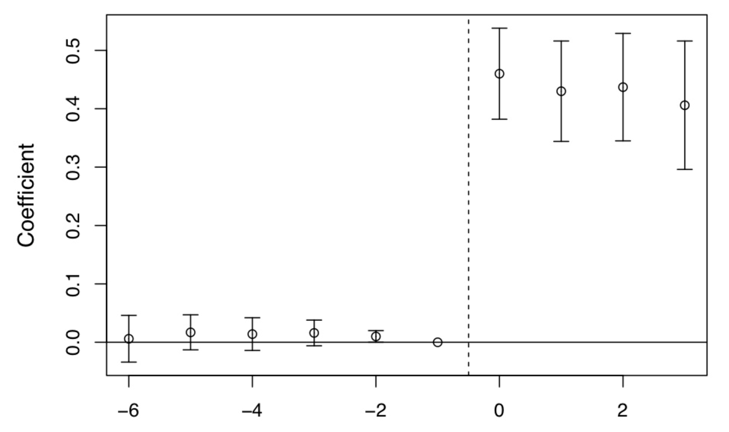
- $\gamma_{\tau}$ captures pre‑treatment parallel trends. It should be approximately zero if the parallel trends assumption holds.
- $\delta_{\tau}$ is the treatment effect to be estimated and is expected to be non‑zero.
Ideally, the plot of $\gamma_{\tau}$ (left) and $\delta_{\tau}$ (right) should look like this:
3 Placebo falsification
Placebo tests help mitigate two concerns:
- Alternative hypotheses. Keep the same treatment but replace $Y$ with alternative outcomes.
- The validity of statistical significance (p‑values). Use randomization inference.
3.1 Rule out alternative hypotheses
“If we find, using our preferred design, effects where there shouldn’t be, then maybe our original findings weren’t credible.”
Example: minimum wage. Fit the same DD design using high‑wage employment as the outcome. If the coefficient on minimum wages is zero when using high‑wage worker employment as the outcome, but the coefficient for low‑wage workers is negative, this complements the earlier findings for low‑wage workers.
Another example is the Medicare expansion–mortality study (Cheng & Hoekstra, 2013).
3.2 Randomization inference
Most useful when there’s only one treatment group
Consider the DD model (randomization inference does not apply to the event study model since it requires only one treatment dummy) with two‑way standard‑error clustering: $$Y_{ist}=\alpha+\lambda_{s}+\lambda_{t}+\delta\times Treat_{s}\times Post_{t}+\beta X_{it}+\varepsilon_{it}$$ Clustering standard errors at the state‑year level assumes constant correlation at that level, yet there may still be severe correlation within a state‑year cell. To do randomization inference:
- Randomly choose a different treatment date (e.g., move the treatment year backward by 1, 2, 3, … years).
- Randomly assign treatment to states. For example, if in the original data 30% are treated and 70% are not, randomly (without replacement) sample 30% as treated.
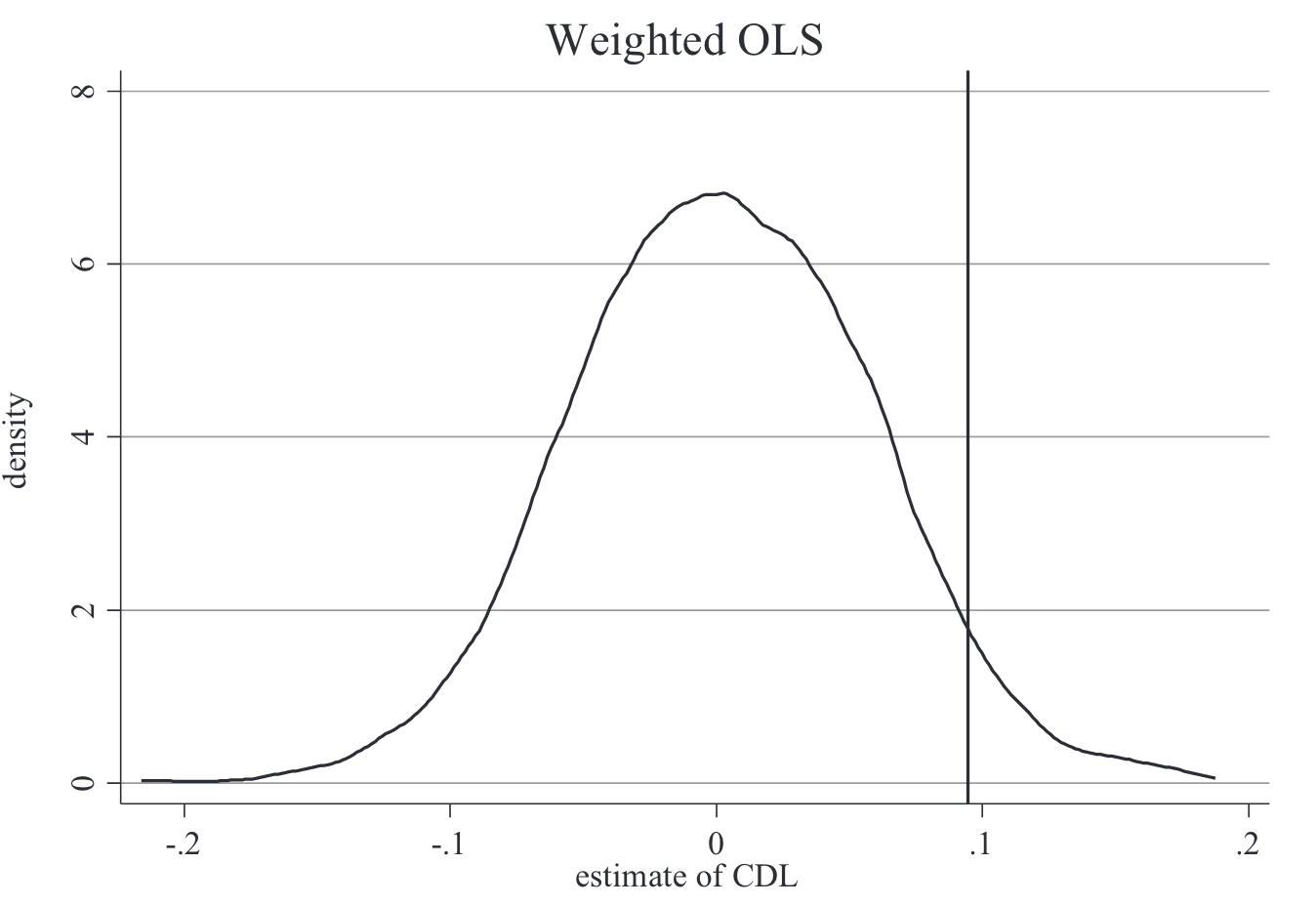
- In total, there are N_date × N_state combinations. Draw a subset at random.
- Plot the p‑value distribution of these placebo estimates and compare with the real one. Example from Cheng & Hoekstra (2013):
width=400
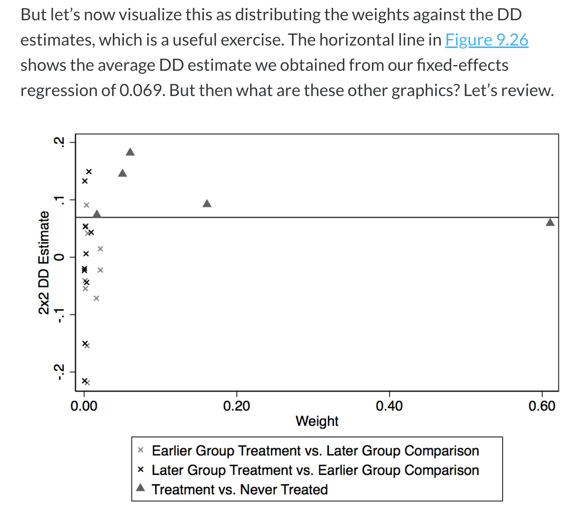
4 Bacon decomposition of two‑way fixed effects
With two‑way fixed effects, the DD estimator aggregates all possible 2×2 comparisons weighted by group shares and treatment variance. The Bacon decomposition reveals a key issue of DD: coefficients on static two‑way FE leads and lags can be unintelligible if treatment effects are heterogeneous over time (Goodman‑Bacon, 2019). In that case, heterogeneity‑induced biases challenge the DD design using two‑way FEs.
In R, use the bacondecomp package. Interpreting its results:
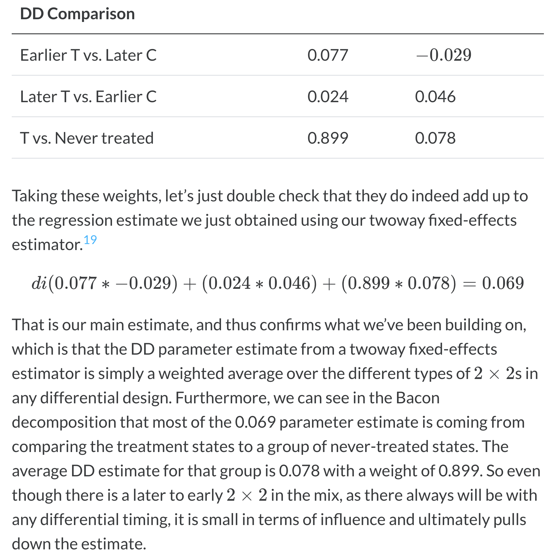
Bacon decomp results