(R) Super Efficient Event Study Code

Yu Zhu included in series R and data.table

2023-05-27 2023-05-27 4310 words 21 minutes

Series -

Contents

Why you want to use this code?

Event study is not new, and there exists plenty of third-party packages to do it, let alone we have WRDS’s official SAS or Python versions. What I’m not satisfied about is that they’re all slow. Here I present a pure R implementation of event study that has the following advantages:

It’s fast. I tested it on a large dataset (3+ millions rows, 3000+ unique stocks, 10k+ events) and it only took 11.4 seconds to compuate the CARs of all these events. If you use WRDS’s SAS version, it may take minutes.
It’s elegant and short. The event study is wrapped up in a single function do_car. The core part of do_car is less than 40 lines.
It replicates WRDS’s version. I compared the result of my code with WRDS’s SAS version, and I found my code fully replicates WRDS.
It’s purely in R.

Before you read it

The full code is in Putting them together.
If you want to add more bells and whistles, see The full-fledged CRSP version. This version includes sanity checks and fast-fail conditions, among many others. You may or may not need them.
The R code I’ll show heavily relies on some advanced techniques of the data.table package. Without data.table (for example, using dplyr only), I can’t achieve the speedup you’ll see later.
IMHO, data.table is much faster than dplyr or pandas in many use cases while requiring 30% or even 50% less code. It encourages you to think selecting, column modification, and grouping operations as a single elegant, coherent operation, instead of breaking them down. You don’t need to take my word, checkout the official introduction and performance benchmark yourself and you’ll realize it.
You don’t need to be a data.table master to understand this article, but some working knowledge is definitely helpful.

1 The dataset

In this article, we’ll build a highly efficient event study program in R. We’ll use all the earnings call events in 2021 in the CRSP stock universe as an example. events is the only dataset we’ll use in this example. Each row of it records the daily return and an event flag: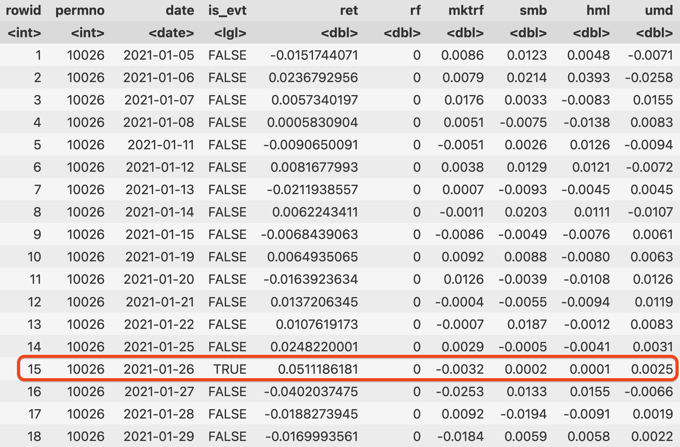

date: all the available trading dates for the stock in a ascending order.
is_evt: True if date is an event date (in our case, earnings call day) and False if it’s an non-event trading day.
ret: daily return of the stock
rf, mktrf, smb, hml, umd: Fama-French factors plus momentum. You can add more as you like.

Requirement of the input dataset

What’s important about the events table is that it contains both the daily return (which will be used in regression) and an event flag (used to determine the event window).
Usually, we want to include enough pre-event and post-event daily returns. In this sample dataset, I extend each event by 2 years’ of data. That is, if the event date is 2021-01-26, I’ll include all the daily returns (and factor returns) from 2019-01-26 to 2023-01-26. That’s probably more than enough, since most event studies has much smaller windows.
Given an event date, how to extract the daily returns in its surrounding days is a problem. I included the code at the end but leave it to the reader to study it, since our main focus is the event study part.

2 For a single event

Let’s say we want to calculate the CAR to measure the abnormal return during the event period. To start, we focus on this question:

If there’s only one event and one stock, how to write a function to compute the CAR?

I assure you, after understanding the code for one event, extending it to many events is very straightforward.

2.1 Specify the windows

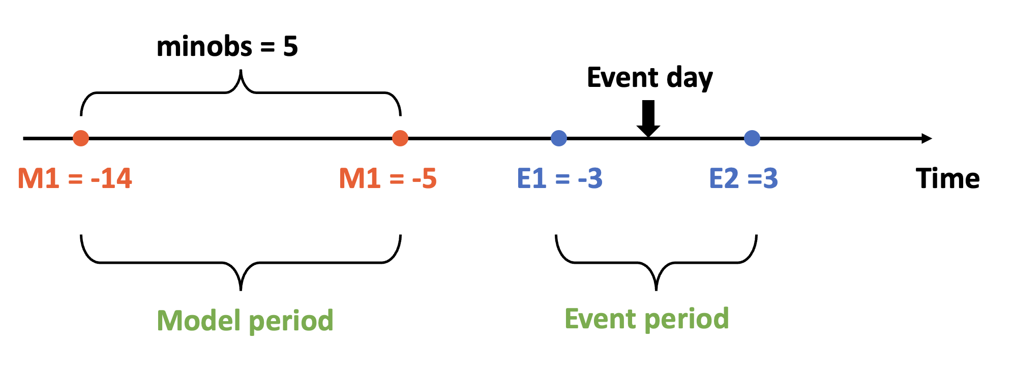
First, let’s specify the windows of our event study, we’ll use the setting throughout this article:

m1 and m2 specify the start and end day of the model period (“m” stands for model). Model period is used to estimate the expected return model. In this example, we use (-14, -5). This is shorter than a typical event study, but it makes our later illustration convenient.
minobs specifies the minimal trading days in the model period. In this example, we require a stock must have no less than 5 trading days before the event.
e1 and e2 specify the event period, i.e., the window during which CAR (cumulative abnormal return) is calculated (“e” stands for event). In this example, we compute CAR from the previous 3 trading day to the following 3 trading days, i.e., CAR(-3,3).
Event day took place on day 0.

Conventionally, the event time is counted as “trading day” instead of “calendar day”

2.2 `do_car`: the core function

do_car is core of the program. For every event, it 1) estimate the expected return model, and 2) compute the abnormal return for each event day. The output looks like:

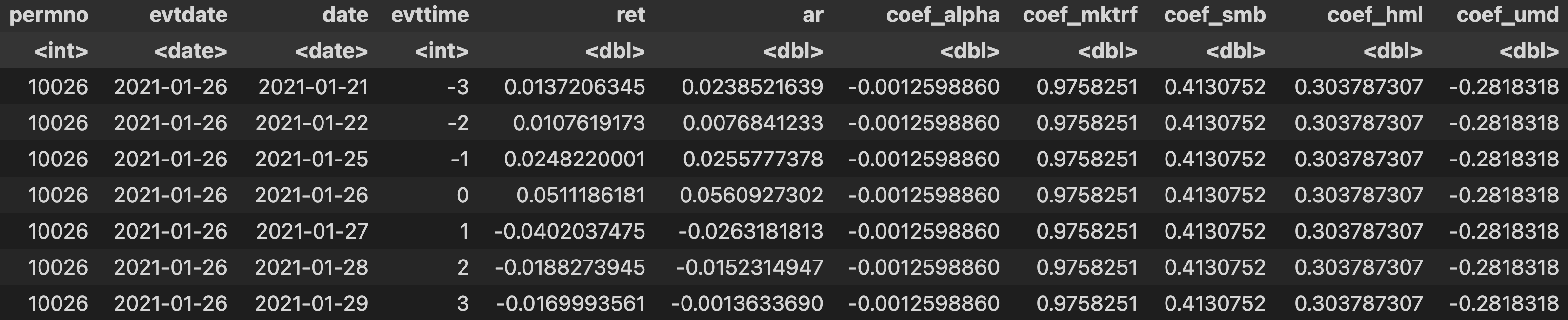
permno, evtdate, date, ret: these columns are already explained above.
evttime: event time indicator, generated by do_car. It equals 0 for the event day. You can see that because the evtdate is 2021-01-26, only date with the same value (2021-01-06) has an evttime of 0.
coef_[alpha/mktrf/smb/hml/umd]: coefficients of the intercept term and factor returns. For the same event (i.e., for a single evtdate), the coefficients are the same, because we only need to estimate one model.
ar: daily abnormal return.

Now let’s a look at the do_car function:

 1
 2
 3
 4
 5
 6
 7
 8
 9
10
11
12
13
14
15
16
17
18
19
20
21
22
23
24
25
26
27
28
29
30
31
32
33
34
35
36
37
38
39
40
41
42
43
44
45
46
47
48
49
50
51
52
53
54
55
56
57
58
59
60
61
62
63
64
65
66
67
68
69
70
71
do_car = function(
    evt_rowidx, permno, date,
    m1, m2, e1, e2, minobs,
    ret, rf, mktrf, smb, hml, umd) {

    # Args:
    #   evt_rowidx: the row number of "one" event in a "permno" group
    #   permno: the "permno" column in the "events" table (for debugging purpose)
    #   date: the "date" column in the "events" table
    #   m1, m2, e1, e2: parameters for the CAR model. "m" stands for model, 
    #     "e" stands for event. 
    #   minobs: minimum number of observations required for the regression
    #   ret: the "ret" or "retx" column in the "events" table
    #   rf, mktrf,..., etc: the factor columns in the "events" table

    # check: nobs >= minobs
    if (evt_rowidx - m1 <= minobs) {
        return(NULL)
    }

    # get indices of model and event windows
    i1 = evt_rowidx - m1
    i2 = evt_rowidx - m2
    i3 = evt_rowidx - e1
    i4 = evt_rowidx + e2

    # (model window) get returns and factors
    ret_model = ret[i1:i2]
    rf_model = rf[i1:i2]
    mktrf_model = mktrf[i1:i2]
    smb_model = smb[i1:i2]
    hml_model = hml[i1:i2]
    umd_model = umd[i1:i2]

    # check: nobs >= minobs (again)
    if (length(ret_model) < minobs) {
        return(NULL)
    }

    # (event window) get returns and factors
    ret_evt = ret[i3:i4]
    rf_evt = rf[i3:i4]
    mktrf_evt = mktrf[i3:i4]
    smb_evt = smb[i3:i4]
    hml_evt = hml[i3:i4]
    umd_evt = umd[i3:i4]

    # get evttime (0 if event day, 1 if day after event, etc.)
    evtdate = date[evt_rowidx]
    evttime = seq(-e1, e2)
    date_evt = date[i3:i4]

    # run regression
    model = lm(I(ret_model-rf_model) ~ mktrf_model + smb_model + hml_model + umd_model)

    # get coefficients
    coef = coef(model)
    coef_names = names(coef)
    
    # rename coefficients
    coef_names = coef_names %>% str_replace_all(c('_model'='', '\\(Intercept\\)'='alpha'))
    coef_names = str_c('coef_', coef_names)
    names(coef) = coef_names

    # get abnormal returns
    ars = ret_evt - predict(model, list(ret_model=ret_evt, rf_model=rf_evt, mktrf_model=mktrf_evt, smb_model=smb_evt, hml_model=hml_evt, umd_model=umd_evt))

    # collect output
    output = list(evtdate=date[evt_rowidx], date=date_evt, evttime=evttime, ret=ret_evt, ar = ars)
    output = c(output, coef)
}

Most of the inputs are no strangers to us, for they’re simply columns from the events table as we explained before. We’ll use the dataset we introduced earlier to explain what do_car does. Let’s assume the following table contains the full sample, i.e., there’re only 18 rows (days), and the event took place on 2021-01-26 (the 15th row):

For do_car, the inputs are:

evt_rowidx (event row index). It’s the row index of the event in the table. In our case, it’s 15 because event date is the 15th row.
permno, date, ret, rf, mktrf, smb, hml, umd are simply columns from the table. For example, permno=[10026, 10026, ...], date=[2021-01-05, ..., 2021-01-29].
m1, m2, e1, e2 and minobs specify the model period and event period. See Specify the windows

Now let’s look at what do_car exactly does. The general idea is simple: we first extract the time series that will be used for the model period (i.e., m1 to m2) and the event period (i.e., e1 to e2), respectively. We then estimate the model on the model period. Finally, we apply the model to the window period and calculate the abnormal return.

Specifically (if you lose track, read this figure again):

We create four “indicators”: i1 to i4. They help us to extract the time series needed. In our example, i1=evt_rowidx+m1=15+(-14)=1, i2=evt_rowidx+m2=15+(-5)=10, therefore, the model period is from the 1st row to the 10th row. To get the daily return of the model period, we simply run ret_model=ret[i1:i2]. Similarly, we can get the time series of the factor returns by smb_model=smb[i1:i2], hml_model=hml[i1:i2], etc.
Similarly, we can calculate the time indicators for the “event period”: i3 and i4. We use them to get the time series for the event period: ret_evt=ret[i3:i4], hml_evt=evt[i3:i4], etc.
Now, we can estimate the expected return model: model = lm(I(ret_model-rf_model) ~ mktrf_model + smb_model + hml_model + umd_model)
We save its coefficients with coef = coef(model)
We then apply the model to the event period and calculate the abnormal returns: ars = ret_evt - predict(model, list(ret_model=ret_evt, rf_model=rf_evt, mktrf_model=mktrf_evt, smb_model=smb_evt, hml_model=hml_evt, umd_model=umd_evt))
Finally, we assemble the results (the coefficients and the abnormal returns) into a table:
- output = list(evtdate=date[evt_rowidx], date=date_evt, evttime=evttime, ret=ret_evt, ar = ars)
- output = c(output, coef)

3 Scale to many events

As I said before, after you know how to compute for one event, extending to thousands of events is straightforward. All you need is:

 1
 2
 3
 4
 5
 6
 7
 8
 9
10
11
12
13
events[, {
    # get event row indices
    evt_rowidxs = which(is_evt)

    # loop over events
    lapply(evt_rowidxs, 
            partial(do_car, permno=permno[1], date=date, ret=ret, rf=rf, mktrf=mktrf,
                    smb=smb, hml=hml, umd=umd, m1=m1, m2=m2, e1=e1,
                    e2=e2, minobs=minobs)
    ) %>% rbindlist()
    },
    keyby=.(permno)
]

Some of lines you’re already familiar with:

do_car is exactly the same function we developed in "do_car the core function"
events is the input dataset we introduced in The dataset. It contains all the earnings calls in 2021.

What’s new is:

The keyby= argument at the end. If you ignore the strange code in the middle, the structure of the above code is:

1
2
3
4
5
events[, {
	...
	},
	keyby=.(permno)
]

As you can see, keyby “groups” the dataset by the permno column. If you come from dplyr, it equals to group_by; if you come from pandas, it’s df.groupby
The keyby argument is executed before the middle code {...} wrapped by curly braces. Therefore, the middle {...} only needs to deal with one stock now (though it can have many events).

Now let’s look at what’s in the middle curly braces {...}. We excerpt this part as follows:

 1
 2
 3
 4
 5
 6
 7
 8
 9
10
11
	{
    # get event row indices
    evt_rowidxs = which(is_evt)

    # loop over events
    lapply(evt_rowidxs, 
            partial(do_car, permno=permno[1], date=date, ret=ret, rf=rf, mktrf=mktrf,
                    smb=smb, hml=hml, umd=umd, m1=m1, m2=m2, e1=e1,
                    e2=e2, minobs=minobs)
    ) %>% rbindlist()
	}

evt_rowidxs = which(is_evt) returns all the event row indexes of for the given permno (remember we’re now working with only one stock before we already keyby=). For example, if it returns c(101, 450), then it means there’re two events on row 101 and 450.
In do_car, we only dealt with one event, but now evt_rowidxs gives us many events. We use lapply(evt_rowidx, do_car) to apply do_car to each event in evt_rowidx.
But do_car has many input arguments (e.g., evt_rowidx, hml, smb, etc.), and evt_rowidx can only provide one: evt_rowidx. To successfully lapply, we need to first fill up the other arguments before sending do_car to lapply. That’s what partial does. It “pre-fill” arguments of a function.

partial is from the pryr package. If you’ve read Hadley Wickham’s Advanced R, you won’t be strange to pryr. Because he created this package and used it a lot in the book.

As the “l” in its name indicates, lapply returns a “list” of results, with each element for one event. To convert the list of results into a 2D table, we used rbindlist (row-bind-list).

Congrats! Now you’ve grasped a super efficient event study program!

3.1 Putting them together

The full code is provided below. It assumes you already have the input data as detailed in the beginning and the window specifications detailed in this figure. The output is like this figure.

 1
 2
 3
 4
 5
 6
 7
 8
 9
10
11
12
13
14
15
16
17
18
19
20
21
22
23
24
25
26
27
28
29
30
31
32
33
34
35
36
37
38
39
40
41
42
43
44
45
46
47
48
49
50
51
52
53
54
55
56
57
58
59
60
61
62
63
64
65
66
67
68
69
70
71
72
73
74
75
76
77
78
79
80
81
82
83
84
85
86
87
88
89
90
91
92
93
94
95
96
97
98
library(data.table)
library(pryr)
library(magrittr)  # for the "%>%" sign.

# do_car process one event
do_car = function(
    evt_rowidx, permno, date,
    m1, m2, e1, e2, minobs,
    ret, rf, mktrf, smb, hml, umd) {

    # Args:
    #   evt_rowidx: the row number of "one" event in a "permno" group
    #   permno: the "permno" column in the "events" table (for debugging purpose)
    #   date: the "date" column in the "events" table
    #   m1, m2, e1, e2: parameters for the CAR model. "m" stands for model, 
    #     "e" stands for event. 
    #   minobs: minimum number of observations required for the regression
    #   ret: the "ret" or "retx" column in the "events" table
    #   rf, mktrf,..., etc: the factor columns in the "events" table

    # check: nobs >= minobs
    if (evt_rowidx - m1 <= minobs) {
        return(NULL)
    }

    # get indices of model and event windows
    i1 = evt_rowidx - m1
    i2 = evt_rowidx - m2
    i3 = evt_rowidx - e1
    i4 = evt_rowidx + e2

    # (model window) get returns and factors
    ret_model = ret[i1:i2]
    rf_model = rf[i1:i2]
    mktrf_model = mktrf[i1:i2]
    smb_model = smb[i1:i2]
    hml_model = hml[i1:i2]
    umd_model = umd[i1:i2]

    # check: nobs >= minobs (again)
    if (length(ret_model) < minobs) {
        return(NULL)
    }

    # (event window) get returns and factors
    ret_evt = ret[i3:i4]
    rf_evt = rf[i3:i4]
    mktrf_evt = mktrf[i3:i4]
    smb_evt = smb[i3:i4]
    hml_evt = hml[i3:i4]
    umd_evt = umd[i3:i4]

    # get evttime (0 if event day, 1 if day after event, etc.)
    evtdate = date[evt_rowidx]
    evttime = seq(-e1, e2)
    date_evt = date[i3:i4]

    # run regression
    model = lm(I(ret_model-rf_model) ~ mktrf_model + smb_model + hml_model + umd_model)

    # get coefficients
    coef = coef(model)
    coef_names = names(coef)
    
    # rename coefficients
    coef_names = coef_names %>% str_replace_all(c('_model'='', '\\(Intercept\\)'='alpha'))
    coef_names = str_c('coef_', coef_names)
    names(coef) = coef_names

    # get abnormal returns
    ars = ret_evt - predict(model, list(ret_model=ret_evt, rf_model=rf_evt, mktrf_model=mktrf_evt, smb_model=smb_evt, hml_model=hml_evt, umd_model=umd_evt))

    # collect output
    output = list(evtdate=date[evt_rowidx], date=date_evt, evttime=evttime, ret=ret_evt, ar = ars)
    output = c(output, coef)
}

# window specifications
m1 = -14
m2 = -5
e1 = -3
e2 = 3
minobs = 5

# run do_car for each permno
events[, {
    # get event row indices
    evt_rowidxs = which(is_evt)

    # loop over events
    lapply(evt_rowidxs, 
            partial(do_car, permno=permno[1], date=date, ret=ret, rf=rf, mktrf=mktrf,
                    smb=smb, hml=hml, umd=umd, m1=m1, m2=m2, e1=e1,
                    e2=e2, minobs=minobs)
    ) %>% rbindlist()
    },
    keyby=.(permno)
]

The efficiency of "do_car"

I test the above code on the dataset we introduced in the beginning–all earnings call events of the whole CRSP universe in 2021. It has 3.16 million row, 3179 unique stocks, 10229 unique events. By no means it’s small.
It only took 11.4 seconds to compute!

4 The full-fledged CRSP version

The code I showed above definitely does what it’s supposed to do. However, if you want to add some bells and whistles, refer to the full-fledge version below. With the knowledge you already know, they’re not so hard to understand.

The full-fledged version:

Include code to generate the input dataset events, i.e., it contains a function get_retevt to extract daily returns data for each event.
Fully based on CRSP.
Include many sanity checks for fast-fail and debugging.

  1
  2
  3
  4
  5
  6
  7
  8
  9
 10
 11
 12
 13
 14
 15
 16
 17
 18
 19
 20
 21
 22
 23
 24
 25
 26
 27
 28
 29
 30
 31
 32
 33
 34
 35
 36
 37
 38
 39
 40
 41
 42
 43
 44
 45
 46
 47
 48
 49
 50
 51
 52
 53
 54
 55
 56
 57
 58
 59
 60
 61
 62
 63
 64
 65
 66
 67
 68
 69
 70
 71
 72
 73
 74
 75
 76
 77
 78
 79
 80
 81
 82
 83
 84
 85
 86
 87
 88
 89
 90
 91
 92
 93
 94
 95
 96
 97
 98
 99
100
101
102
103
104
105
106
107
108
109
110
111
112
113
114
115
116
117
118
119
120
121
122
123
124
125
126
127
128
129
130
131
132
133
134
135
136
137
138
139
140
141
142
143
144
145
146
147
148
149
150
151
152
153
154
155
156
157
158
159
160
161
162
163
164
165
166
167
168
169
170
171
172
173
174
175
176
177
178
179
180
181
182
183
184
185
186
187
188
189
190
191
192
193
194
195
196
197
198
199
200
201
202
203
204
205
206
207
208
209
210
211
212
213
214
215
216
217
218
219
220
221
222
223
224
225
226
227
228
229
230
231
232
233
234
235
236
237
238
239
240
241
242
243
244
245
246
247
248
249
250
251
252
253
254
255
256
257
258
259
260
261
262
263
264
265
266
267
268
269
270
271
272
# Step 1: get the "ret-event" table. 
# This table contains the following columns:
#   - permno, date: identifiers
#   - is_event: boolean, if the "date" is an event date or not
#   - ret: raw daily return of the stock, including dividends
#   - rf, mktrf, umd, smb, hml, cma, rmw: FF5 factors plus momentum
get_retevt = function(events) {
    # Args:
    #   events: a data.table of (permno, evtdate) pairs. If NULL, we read from the file.

    # step 1: get the "events" table
    # each row is an (permno, evtdate) pair
    events[, ':='(join_date=evtdate)]
    events = unique(events[!is.na(permno) & !is.na(evtdate)])
    unique_permnos = events[, unique(permno)]

    # we extend the sample by 2 years on both sides to make sure the regression window is covered
    syear = events[, min(year(evtdate))]-2  # start year of the sample
    eyear = events[, max(year(evtdate))]+2  # end year of the sample

    # step 2: get the "daily return" table    
    dly_rets= open_dataset('crsp/feather/q_stock_v2/wrds_dsfv2_query', format='feather') %>% 
        select(permno, dlycaldt, dlyret, dlyretx, year) %>%
        filter(year %between% c(syear, eyear), permno %in% unique_permnos, !is.na(permno), !is.na(dlycaldt), !is.na(dlyret), !is.na(dlyretx)) %>%
        transmute(permno, date=dlycaldt, ret=dlyret, retx=dlyretx, join_date=date) %>%
        # head(1) %>% 
        collect() %>%
        as.data.table()

    # step 3: get factors (ff5umd or ff3umd)
    ff5umd = open_dataset('ff/feather/fivefactors_daily.feather', format='feather') %>% 
        transmute(date, ff5umd_rf=rf, ff5umd_mktrf=mktrf, ff5umd_smb=smb, ff5umd_hml=hml, ff5umd_rmw=rmw, ff5umd_cma=cma, ff5umd_umd=umd) %>%
        collect() %>%
        as.data.table()
    ff3umd = open_dataset('ff/feather/factors_daily.feather', format='feather') %>% 
        transmute(date, ff3umd_rf=rf, ff3umd_mktrf=mktrf, ff3umd_smb=smb, ff3umd_hml=hml, ff3umd_umd=umd) %>%
        collect() %>%
        as.data.table()

    # step 4: merge events, dly_rets, and ff factors
    retevt = events[
        # merge events and dly_rets
        dly_rets, on=.(permno, join_date)
        ][!is.na(permno), .(permno, date, ret, retx, is_evt=!is.na(evtdate))
        # merge ff5umd
        ][ff5umd, on=.(date), nomatch=NULL
        # merge ff3umd
        ][ff3umd, on=.(date), nomatch=NULL
        # housekeeping
        ][, .(permno, date, is_evt, ret, retx, 
              ff3umd_rf, ff3umd_mktrf, ff3umd_smb, ff3umd_hml, ff3umd_umd,
              ff5umd_rf, ff5umd_mktrf, ff5umd_smb, ff5umd_hml, ff5umd_rmw, ff5umd_cma, ff5umd_umd)
        ][order(permno, date)]
}

# Step 2: loop through each event

# `do_car` compute the CAR for one event
do_car = function(
    evt_rowidx, permno, date,
    m1, m2, e1, e2, minobs, ff_model,
    ret, rf, mktrf, smb, hml, umd, cma, rmw, return_coef, verbose) {

    # Args:
    #   evtrow: the row number of "one" event in a "permno" group
    #   permno: the "permno" column in the "retevt" table (for debugging purpose)
    #   date: the "date" column in the "retevt" table
    #   m1, m2, e1, e2: parameters for the CAR model. "m" stands for model, 
    #     "e" stands for event. All numbers are converted to positive integers.
    #   minobs: minimum number of observations required for the regression
    #   ff_model: the factor model to use. "ff3", "ff3umd", "ff5", or "ff5umd"
    #   ret: the "ret" or "retx" column in the "retevt" table
    #   rf, mktrf,..., etc: the factor columns in the "retevt" table
    #   return_coef: if TRUE, return the regression coefficients
    #   verbose: if TRUE, print out warnings when obs<minobs

    # check: nobs >= minobs
    if (evt_rowidx - m1 <= minobs) {
        if (verbose) sprintf("WARN: (permno=%s, date=%s) nobs is smaller than minobs (%s).\n", permno, date[evt_rowidx], minobs) %>% cat()
        return(NULL)
    }

    # get indices of model and event windows
    i1 = evt_rowidx - m1
    i2 = evt_rowidx - m2
    i3 = evt_rowidx + e1
    i4 = evt_rowidx + e2

    # (model window) get returns and factors
    ret_model = ret[i1:i2]
    rf_model = rf[i1:i2]
    mktrf_model = mktrf[i1:i2]
    smb_model = smb[i1:i2]
    hml_model = hml[i1:i2]
    umd_model = umd[i1:i2]
    if (!is.null(cma)) cma_model = cma[i1:i2]
    if (!is.null(rmw)) rmw_model = rmw[i1:i2]

    # check: nobs >= minobs (again)
    if (length(ret_model) < minobs) {
        if (verbose) sprintf("WARN: (permno=%s, date=%s) nobs is smaller than minobs (%s).\n", permno, date[evt_rowidx], minobs) %>% cat()
        return(NULL)
    }

    # (event window) get returns and factors
    ret_evt = ret[i3:i4]
    rf_evt = rf[i3:i4]
    mktrf_evt = mktrf[i3:i4]
    smb_evt = smb[i3:i4]
    hml_evt = hml[i3:i4]
    umd_evt = umd[i3:i4]
    if (!is.null(cma)) cma_evt = cma[i3:i4]
    if (!is.null(rmw)) rmw_evt = rmw[i3:i4]

    # get evttime (0 if event day, 1 if day after event, etc.)
    evtdate = date[evt_rowidx]
    evttime = seq(-e1, e2)
    date_evt = date[i3:i4]

    # check: length of output variables are the same
    stopifnot(length(ret_evt)==length(evttime), length(ret_evt)==length(date_evt))

    # # debug only
    # if (all(is.na(ret_model))) {
    #     print(evtdate)
    #     print(permno)
    # }
        
    # run regression
    if (ff_model == 'ff3') {
        model = lm(I(ret_model-rf_model) ~ mktrf_model + smb_model + hml_model)
    } else if (ff_model == 'ff3umd') {
        model = lm(I(ret_model-rf_model) ~ mktrf_model + smb_model + hml_model + umd_model)
    } else if (ff_model == 'ff5') {
        model = lm(I(ret_model-rf_model) ~ mktrf_model + smb_model + hml_model + rmw_model + cma_model)
    } else if (ff_model == 'ff5umd') {
        model = lm(I(ret_model-rf_model) ~ mktrf_model + smb_model + hml_model + rmw_model + cma_model + umd_model)
    } else {
        stop('ff_model must be one of "ff3", "ff3umd", "ff5", or "ff5umd"')
    }

    # get coefficients
    coef = coef(model)
    coef_names = names(coef)
    # rename coefficients
    coef_names = coef_names %>% str_replace_all(c('_model'='', '\\(Intercept\\)'='alpha'))
    coef_names = str_c('coef_', coef_names)
    names(coef) = coef_names

    # get abnormal returns
    if (ff_model == 'ff3') {
        ars = ret_evt - predict(model, list(ret_model=ret_evt, rf_model=rf_evt, mktrf_model=mktrf_evt, smb_model=smb_evt, hml_model=hml_evt))
    } else if (ff_model == 'ff3umd') {
        ars = ret_evt - predict(model, list(ret_model=ret_evt, rf_model=rf_evt, mktrf_model=mktrf_evt, smb_model=smb_evt, hml_model=hml_evt, umd_model=umd_evt))
    } else if (ff_model == 'ff5') {
        ars = ret_evt - predict(model, list(ret_model=ret_evt, rf_model=rf_evt, mktrf_model=mktrf_evt, smb_model=smb_evt, hml_model=hml_evt, rmw_model=rmw_evt, cma_model=cma_evt))
    } else if (ff_model == 'ff5umd') {
        ars = ret_evt - predict(model, list(ret_model=ret_evt, rf_model=rf_evt, mktrf_model=mktrf_evt, smb_model=smb_evt, hml_model=hml_evt, rmw_model=rmw_evt, cma_model=cma_evt, umd_model=umd_evt))
    }

    # collect output
    output = list(evtdate=date[evt_rowidx], date=date_evt, evttime=evttime, ret=ret_evt, ar = ars)
    if (return_coef) output = c(output, coef)
    output
}

# `main` compute CARs for all events in the "retevt" table
main <- function(retevt, m1, m2, e1, e2, ret_type, ff_model, minobs, return_coef=F, verbose=F) {
    # Args:
    #    retevt: a data.table containg the returns, factors, and event dates
    #    m1: model window start, e.g. -252
    #    m2: model window end, e.g. -100
    #    e1: event window start, e.g. -10
    #    e2: event window end, e.g. 10
    #    ret_type: one of "ret" or "retx"
    #    ff_model: one of "ff3", "ff3umd", "ff5", or "ff5umd"
    #    minobs: minimum number of observations in the model window
    #    return_coef: if TRUE, return the regression coefficients
    #    verbose: if TRUE, print warnings
    #
    # Returns:
    #     a data.table containing the following columns:
    #         permno, evtdate, date, evttime, ret, base_ret, ar, 
    #         (if return_coef) coef_alpha, coef_mktrf, coef_smb, coef_hml, coef_umd, coef_rmw, coef_cma

    # sanity check of hparams
    stopifnot(m1<m2, m2<=e1, e1<=e2)
    stopifnot(e1<=0, e2>=0)
    stopifnot((m2-m1+1)>=minobs)
    stopifnot(ret_type %in% c('ret', 'retx'))
    stopifnot(ff_model %in% c('ff3', 'ff3umd', 'ff5', 'ff5umd'))

    # convert m1, m2, e1, e2 to positive integers
    m1 = abs(m1)
    m2 = abs(m2)
    e1 = e1
    e2 = e2

    # compute CARs
    result = retevt[, {
        # get returns
        if (ret_type=='ret') {
            ret = ret
        } else if (ret_type=='retx') {
            ret = retx
        }

        # get factors
        if (str_detect(ff_model, 'ff3')) {
            rf = ff3umd_rf
            mktrf = ff3umd_mktrf
            smb = ff3umd_smb
            hml = ff3umd_hml
            umd = ff3umd_umd
            cma = NULL
            rmw = NULL
        } else if (str_detect(ff_model, 'ff5')) {
            rf = ff5umd_rf
            mktrf = ff5umd_mktrf
            smb = ff5umd_smb
            hml = ff5umd_hml
            rmw = ff5umd_rmw
            cma = ff5umd_cma
            umd = ff5umd_umd
        }

        # get event row indices
        evt_rowidxs = which(is_evt)

        # loop over events
        lapply(evt_rowidxs, 
               partial(do_car, permno=permno[1], date=date, ret=ret, rf=rf, mktrf=mktrf,
                       smb=smb, hml=hml, rmw=rmw, cma=cma, umd=umd, m1=m1, m2=m2, e1=e1,
                       e2=e2, minobs=minobs, ff_model=ff_model, return_coef=return_coef,
                       verbose=verbose)
        ) %>% rbindlist()
        },
        
        # group by permno
        keyby=.(permno)

    # compute base returns
    ][, ':='(base_ret=ret-ar)][]
}

# ---- hparams ----
# Translation from WRDS's evtstudy to my version:
#    WRDS (default): estwin=100, gap=50, evtwins=-10, evtwine=10, minval=70
#    My version, m1=evtwins-gap-estwin, m2=evtwins-gap-1, 
#                e1=evtwins, e2=evtwine, minobs=minval
m1 = -252
m2 = -31
e1 = -30
e2 = 252
minobs = 70  # minimum number of observations in the regression

ret_type = 'ret'  # 'ret' or 'retx'
ff_model = 'ff5umd'  # 'ff3', 'ff3umd', 'ff5', or 'ff5umd

# ---- Step 1: get the "return-events" table -----
events = list()
for (year in 2007:2021) {
    evt = fread(paste0('~/OneDrive/Call/local-dev/data/v2/ars/event_dates/carday0_call/', year, '.csv'))
    events[[year]] = evt[, .(permno, evtdate=edate)]
}
events = rbindlist(events)
retevt = get_retevt(events)
sprintf('Number of events: %d\n', retevt[, sum(is_evt)]) %>% cat()

# ---- Step 2: compute CARs ----
result = main(retevt=retevt, m1=m1, m2=m2, e1=e1, e2=e2, ret_type=ret_type, ff_model=ff_model, minobs=minobs, return_coef=T, verbose=F)
write_feather(result, sprintf('~/OneDrive/Call/local-dev/data/v2/ars/ars_%s_call_raw.feather', ff_model))